Concepts in Knowledge Graphs

Notes on reading the long survey: Knowledge Graphs (see References).

Knowledge Graph

A graph of data intended to accumulate and convey knowledge of the real world, whose nodes represent entities of interest and whose edges represent relations between these entities.
Interpretation

Mapping the nodes and edges in the data graph to those (respectively) of the domain graph.
Model

The interpretations that satisfy a graph are called models of the graph.
Entailment

One graph entails another iff any model of the former graph is also a model of the latter graph.
Graph Pattern

Data graphs allowing variables as terms.
Inference Rules

A rule encodes IF-THEN style consequences and is composed of a body (IF) and a head (THEN), both of which are given as graph patterns.
Materialisation

Refers to the idea of applying rules recursively to a graph, adding the conclusions generated back to the graph until a fixpoint is reached and nothing more can be added.
Query Rewriting

Automatically extends the query in order to find solutions entailed by a set of rules.
Description Logics

DLs are based on three types of elements: individuals (e.g. Santiago); classes (e.g. City); and properties (e.g. flight). DLs then allow for making claims, known as axioms, about these elements. Assertional axioms form the Assertional Box (A-Box); Class axioms form the Terminology Box (T-Box); Property axioms form the Role Box (R-Box). ⊤ symbol is used in DLs to denote the class of all individuals.
Deductive vs. Inductive

Deductive knowledge is characterised by precise logicial consequences; Inductive knowledge involves generalising patterns (then making predictions with a level of confidence) from observations.
Supervised, Self-supervised and Unsupervised Methods

Supervised methods learn a function (model) to map a given set of example inputs to their labelled outputs; Self-supervisision rather finds ways to generate the input-output pairs automatically from the input, then fed into a supervised process to learn a model; Unsupervised processes do not require lablled input-output pairs, but rather apply a predefined function to map inputs to outputs.
Graph Analytics

Analytics is the process of discovering, interpreting, and communicating meaningful patterns inherent to data collections (graph data for Graph Analytics). Topology of the graph is how the nodes of the graph are connected.

12.1 Main techniques: Centrality aiming to identify the most important nodes or edges of the graph. Community detection aiming to identify communities, i.e. sub-graphs that are more densely connected internally than to the rest of the graph; Connectivity aiming to estimate how well-connected the graph is, revealing, e.g. the resilience and (un)reachability of elements of the graph; Node similarity aiming to find nodes that are similar to other nodes by virtue of how they are connected within their neighbourhood; Path finding aiming to find paths in a graph, typically between pairs of nodes given as input.

12.2 Graph parallel frameworks apply a systolic abstraction where nodes are processors that can send message to other nodes along edges; an algorithm in this framework consists of the functions to compute message values in the message phase (MsG), and to accumulate the messages in the aggregation phase (AGG); additional features including global step (global computation) and mutation step (adding/removing during processing).

12.3 Analytics involving edge meta-data: Projection drops all edge metat-data; Weighting converts edge meta-data into numerical values according to some function; Transformation involves transforming the graph to a lower arity model, where being lossy means irreversible transformation (lossing information) and being lossless means reversible; Customisation involves changing the analytical procedure to incorporate edge meta-data.

Note: The combination of analytics and entailment, according to the survey, has not been well-explored.
Knowledge Graph Embeddings

Embedding is given by some mathematical function \(f: X \rightarrow Y\) which is injective, structure-preserving and often maps from the abstract high dimensional space to the concrete low diemnsional space to resolve the sparsity and fractured information caused by one-hot encoding. Here \(X\) is said to be embedded in \(Y\). The main goal is to create a dense representation of teh graph in a continuous, low-dimensional vector space, where the dimensionality d is typically low, e.g. \(50 \leq d \leq 1000 \).

13.1 Most common instantiation is given an edge \([s] \xrightarrow{p} [o] \), and the embeddings \(e_s, r_p, e_o\) (e stands for entity, r stands for relation), the scoring function computes the plausibility of the edge. The goal is then to compute the embeddings that maximise the plausibility of postive edges (typically edges in the graph) and minimise the plausibility of negative examples (typically edges in the graph with a node or edge label changed) according to the scoring function. The resulting embeddings can be seen as encoding latent features of graph through self-supervision, mapping input edges to output plausibility scores.

13.2 Translational models interpret edge labels as transformations from subject nodes (source, head) to object nodes (target, tail). The most elementary approach is TransE, aiming to make \(e_s + r_p \rightarrow e_o\) for positive edges \([s] \xrightarrow{p} [o] \), and keeps the sum away from \(e_o\) for negative examples. TransE tends to assign cyclical relations a zero vector as the directional components will tend to cancel each other out. Variants of TransE such as TransH (represents different relations using distinct hyperplanes, so project the \([s]\) onto the hyperplane of \(\xrightarrow{p}\) before translating to \([o]\)), TransR (projects \([s], [o]\) into a vector space specific to \(\xrightarrow{p}\), TransD (simplifies TransR by associating entities and relations with a second vector, where these secondary vectors are used to project the entity into a relation-specific vector space).

13.3 Tensor decomposition models: the original tensor is decomposed into more elementary tensors which capture latent factors (underlying information). Rank decomposition such that \(\sum^r_{i=1} \mathbf{x_i} \otimes \mathbf{y_i} = \mathbf{C} \) is approximated by setting a limit \( d < r\), \(\otimes\) refers to the outer product of vectors (\(\mathbf{x} \otimes \mathbf{y} = \mathbf{x}\mathbf{y^T}\). Method is called Canonical Polyadic (CP) decomposition. For graphs, we can have it encoded as a one-hot, order-3 tensor \(G\) with \(\vert V \vert \times \vert L \vert \times \vert V \vert \) elements, where \(G_{ijk}\) is set to one if \(i^{th}\) node links to \(k^{th}\) node with an edge having \(j^{th}\) label, or zero otherwise. Apply CP we obtain \( \sum^d_{i=1} \mathbf{x_i} \otimes \mathbf{y_i} \otimes \mathbf{z_i} \approx G\) and the decomposed \(\mathbf{x_i}, \mathbf{y_j}, \mathbf{z_k}\) are the graph embeddings we want.

Note: According to the survey, the current state-of-the-art decomposition method is TuckER with \( G = \mathcal{T} \otimes \mathbf{A} \otimes \mathbf{B} \otimes \mathbf{C}\), where the tensor \(\mathcal{T}\) is the “core” tensor.

13.4 Neural models: One of the earliest proposal is Semantic Matching Energy (SME) which learns parameters for two functions such that \(f_s(e_s, r_p) \cdot g_{w’}(e_o, r_p)\) gives the plausibility score; Anoter early work was Neural Tensor Networks (NTN), which proposes to maintain a tensor \(\mathcal{W}\) of internal weights such that the plausibility score is given by a complex function that combines \(e_s \otimes \mathcal{W} \otimes e_o \rightarrow NN_{e_s}, NN_{e_o} \rightarrow r_p\). Multi-layer Perceptron (MLP) is a simpler model, where \(e_s, r_p, e_o\) are concatenated and fed into a hidden layer to compute plausibility score. For more neural models, please refer to page 41 - 42 of the survey.

13.5 Language models: RDF2Vec performs biased random work on the graph and records the paths as sentences, which are then fed as input to word2vec model. KGloVe uses personalised PageRank to determine the most related nodes to a given node, whose results are fed into the GloVe model.

13.6 Entailment-aware models: Use deductive knowledge (ontology, set of rules) to refine the predictions made by embeddings.
Graph Neural Network

14.1 Recursive GNN (RecGNN) takes as input a directed graph where nodes and edges are associated with feature vectors that capture node and edge labels, weights, etc. Each node is associated with state vecotr, which is recursively updated based on neighbours, with convergence up to a fixpoint.

14.2 Convolutional GNN (ConvGNN) has its transition function applied over a node and its neighbours, while for CNN it is appliedon a pixel and its neighbours in the image. One challenge is that neightbours of different nodes can be diverse and approaches to address that involves spectral or spatial representations. An alternative is to use attention mechanism to learn the nodes whose features are most important to the current node.
Symbolic Learning

Previous neural approaches are unable to provide results for edges involving unseedn nodes or edges (out-of-vbocabulary problem) and the models are often difficult to explain. Symbolic learning aims to learn hypotheses in a symbolic (logical) language that “explain” a given set of postive and negative edges.

15.1 Rule mining: The goal is to identify new rules that entail a high ratio of positive edges from other positive edges, but entail a low ratio of negative edges from positive edges. Edges entailed by a rule and a set of positivbe edges are the positive entailments of that rule. The number and the ratio of positive entailments are support and confidence for the rule (good for high support and confidence). Under the Partial Completeness Assumption (PCA), negative examples are edges (\([s] \xrightarrow{p} [o’] \)) NOT in the graph but \(\exists [o]. [s] \xrightarrow{p} [o]\). Edges that are neither positive or negative are ignored by the measure. Rules are closed meaning that each variable appears in at least two edges of the rule, which ensures rules are safe, meaning that each variable in the head appears in the body (see Definition 6 for the concept of head and body). Technique that involves NN is called differentiable rule mining.

15.2 Axiom mining: Axioms are expressed in logicial languages such as DLs.
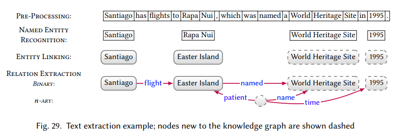
Text Sources

16.1 Pre-processing includes Tokenisation, Part-of-Speech tagging, Depdency Parsing (extracts a grammatical tree structure), Word Sense Disambiguation (to identify sense and link words with a lexicon of senses, e.g. WordNet).

16.2 Named Entity Recognition: Names entities identified by NER may be used to generate new candidate nodes from the KG, or linked to exsisting nodes.

16.3 Entity Linking: Challenging because \([1]\) there are multiple ways to mention the same entity and \([2]\) the same mention in different contexts can refer to distinct entities.

16.4 Relation Extraction: The RE task extracts relations between entities in the text.

References

Hogan, A., E. Blomqvist, Michael Cochez, Claudia D’amato, Gerard de Melo, C. Gutiérrez, J. L. Gayo, S. Kirrane, S. Neumaier, A. Polleres, R. Navigli, Axel-Cyrille Ngonga Ngomo, S. M. Rashid, A. Rula, Lukas Schmelzeisen, Juan Sequeda, Steffen Staab and A. Zimmermann. “Knowledge Graphs.” ArXiv abs/2003.02320 (2020): n. pag.