Introduction
The softmax function is widely used in the output layer of the neural network based model when we have a classification problem. It is the generalization of the sigmoid function in the multi-dimensional space. To see that, suppose we have a random variable \(X\) with only two possible outcomes \(\{ x_1, x_2 \}\), then by applying the softmax function on \(X\), we have:
\[P(X=x_1) = \frac{\exp(x_1)}{\sum_{i=1, 2} \exp(x_i)} = \frac{\exp(x_1)}{\exp(x_1) + \exp(x_2)} = \frac{1}{1 + \exp(-(x_2 - x_1))} = \sigma (x_1 - x_2)\]where \(\sigma (z) = \frac{1}{1 + \exp(-z)}\) is the sigmoid function. Furthermore, we can actually interpret softmax function in the more general form—if we assume our input \(X\) as the log form of some other variable \(Y\) such that \(x_i = \log y_i\), then
\[P(X = x_i = \log y_i) = \frac{\exp(x_i)}{\sum_{j} \exp(x_j)} = \frac{y_i}{\sum_j y_j}\]which can be deemed as normalizing over the sum of all the log-scale variables. In fact, we can easily transform the probability function that involves a normalizing term to the linear one by applying the inverse function to our inputs (e.g. \(\log(\cdot) = \exp^{-1}(\cdot)\)). Taking the natural \(log\) is the assumption made by the logistic model.
Note: In this post, the \(log\) sign is by default of base \(e\) except in the case of binary tree where a base \(2\) is used.
Compared to other types of normalization, the softmax function assigns more extreme probabilities to the outputs, and thus behaving more like the argmax function. Also, because of its differentiability and the nice mathematical properties associated with its gradient, softmax is a good fit for gradient-based optimization such as the stochastic gradient descent.
Nevertheless, the softmax function suffers from the time complexitiy problem resulted from normalizing over the whole vocabulary in the NLP application (e.g. Word2Vec). To deal with it, various approaches for approximating/replacing softmax have been proposed, and this post introduces some of them as well as the maths behind them. Taking the Continuous Bag of Words model as an example, the output conditional probability of predicting the center word \(w\) given the context word \(c\) is given by the softmax function as:
\[P(w | c) = \frac{\exp(S(w, c))}{\sum_{v \in V} \exp(S(v, c)))}\]where \(S(w, c)\) is the scoring function that computes the similarity between the center word \(w\) and the given context word \(c\). To enforce a probability distribution, the softmax function normalizes the exponetial of the similarity score over the whole vocabulary of size \(\lvert V \rvert\), thus requiring a large time consumption (\(O(\lvert V \rvert)\)) when we have a large vocabulary list.
Softmax-based Approaches
The approaches discussed in this section more or less maintain the overall structure of the softmax.
Hierarchical Softmax (H-Softmax)
The idea of H-Softmax starts from manipulating the equation of the conditional probability by partitioning the outcomes of the random variable of interest into clusters. To illustrate, suppose we want to compute the conditional probability of \(Y\) given \(X\), by applying the summation rule we have:
\[P(Y|X) = \sum_k P(Y, C_k | X) = \sum_k P(Y | C_k, X) \cdot P(C_k | X)\]where \(C_k\) stands for the \(k\)th cluster of \(Y\). Suppose there are no overlaps among clusters, we have each \(Y\) corresponding to exactly one cluster \(C(Y)\), thus the probabilities conditioned on other clusters are zeros. Therefore, we can re-write the above equation by discarding the summation symbol as:
\[P(Y|X) = P(Y | C(Y), X) \cdot P(C(Y) | X)\]We can then extend the idea by applying the paritioning recursively as in a binary tree structure such that at each node of the tree, we are partitioning words into two clusters. Suppose we have a balanced binary tree with leaves representing the words in the vocabulary, then the maximum search depth will be \(\log \lvert V \rvert\) instead of \(\lvert V \rvert\) as in the original softmax. Following the previous equation, we can replace the random variables to fit our context as follows:
\[P(w | c) = P(w | p(w), c) \cdot P(p(w) | c)\]where \(p(w)\) stands for the parent node of the leaf for the word \(w\). We can regard \(p(w)\) as the cluster of \(w\) and another word \(w'\) (two children). The recursive step is to merge the cluster \(p(w)\) into a larger cluster by applying the backtracking function \(p(\cdot)\) again and again (climbing up the hierarchy) until reaching the root node (similar to hierarchical k-means). Hence, the final expression is:
\[P(w | c) = \prod_{i=0}^{\log \lvert V \rvert - 2} P(p^i(w) | p^{i+1}(w), c) \cdot P(root)\]where \(p^0(w) = w\), \(P(root) = 1\), and the path is of length \(\log \lvert V \rvert - 1\). The figure below demonstrates an example of computing the conditional probability \(P(blue \vert context)\) in the hierarchical manner.
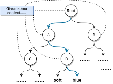
Fig. 1: An example of applying the recursive cluster partitioning as in the balanced binary tree.
Since we are searching in the binary tree, the probability function for each node can be the sigmoid function as proposed in the original work of H-Softmax [2].
Note: Although H-Softmax achieves \(O(\log \lvert v \rvert)\) in training, it still needs to compute the probabilities for all words in testing because we do not know in advance that which word to be predicted (thus we do not know the exact path).
Note: Building a language model for a corpus of vocabulary size \(\lvert V \rvert = 10000\) with a balanced binary tree will result in an overall entropy of \(H = - \sum_{w \in V} p(w) \log p(w) =\)\(- \sum_{w \in V} \frac{1}{\lvert V \rvert} \log \frac{1}{\lvert V \rvert} =\)\(- \log {\lvert V \rvert} \approx 13.3\). However, if we consider the frequencies of words in the corpus, we may have a lower entropy.
Note: The intermediate nodes can be deemed as the latent variables and the performance of H-softmax relies largely on the construction of the tree or the definition of the clusters. One idea is to enforce that similar paths are assigned to similar words.
Differentiated Softmax (D-Softmax)
The idea of D-Softmax was inspired by differentiating words according to their frequencies. Compared to the vanilla softmax with a condense weight matrix in the output layer, D-Softmax utilizes a sparse weight matrix with blocks (of different dimensionalities) distributed to different word embeddings [3].
Character-level Softmax
Instead of having a softmax over the words, we can apply it on the characters sequentially.
Monte-Carlo Sampling Based Approahes
The approaches discussed in this section utilize the Monte-Carlo sampling techniques to approximate the softmax expectation during backpropagation to avoid the expensive computation on the normalizing term. Before delving into the methodology, we need to know some nice mathematical properties of the cross-entropy loss with the softmax activation.
Cross-Entropy Loss with Softmax
In the Word2Vec scenario, the cross-entropy loss for a single instance \(\mathbf{y}\) (one-hot encoding vector with value \(1\) at the \(i\)th position) has the following form (see my previous post here about cross-entropy):
\[L_i = H(\mathbf{y}, \hat{\mathbf{y}}) = - \sum_{j=1}^{\lvert V \rvert} y_j \log \hat{y}_j = - \log \hat{y}_i = - \log \frac{\exp(z_{i})}{\sum_{j=1}^{\lvert V \rvert} \exp(z_j))} = - z_i + \log (\sum_{j=1}^{\lvert V \rvert} \exp(z_j)\]where \(y_j = 1 \iff j=i\) because of the nature of the one-hot encoding, \(z\) refers to the unnormalized result generated from the previous layer, and the output is computed by the softmax activation. In the Word2Vec case (or other context dependent scenarios), \(z_i = S(w_i, c)\) given some context word \(c\). For the clearer illustration of the algebraic calculations, we neglect the context dependence for this section.
Note: The subscripts for \(z\) and \(y\) correspond to the indices of the words in the vocabulary.
Note: The cross-entropy loss happens to be the same as minimizing the negative log-likehood (or MLE) in our scenario.
For backpropagation we need to compute the gradient of the loss as:
\[\begin{aligned} \nabla L_i &= - \nabla z_i + \frac{1}{\sum_{j=1}^{\lvert V \rvert} \exp(z_j)} \cdot \nabla (\sum_{k=1}^{\lvert V \rvert} \exp(z_j))\\ &= - \nabla z_i + \frac{1}{\sum_{j=1}^{\lvert V \rvert} \exp(z_j)} \cdot \sum_{k=1}^{\lvert V \rvert} \nabla \exp(z_k) \\ &= - \nabla z_i + \frac{1}{\sum_{j=1}^{\lvert V \rvert} \exp(z_j)} \cdot \sum_{k=1}^{\lvert V \rvert} \exp(z_k) \nabla z_k\\ &= - \nabla z_i + \sum_{k=1}^{\lvert V \rvert} \frac{\exp(z_k)}{\sum_{j=1}^{\lvert V \rvert} \exp(z_j)} \nabla z_k\\ &= - \nabla z_i + \sum_{k=1}^{\lvert V \rvert} P(z_k) \nabla z_k\\ &= - \nabla z_i + \mathbb{E}[\nabla z] \end{aligned}\]where \(P\) is the softmax probability distribution derived from the network. The final form of the gradient can be deemed as the (negative) deviation from the mean gradient.
Note: The reason for modelling the expectation is that backpropagation does not require the exact loss value and all we need to know is the gradient. However, we need specific softmax value when we want to monitor the convergence of the loss or during the evaluation time.
Monte-Carlo Estimate
The Monte-Carlo estimate of the expectation \(\mathbb{E}[\nabla z]\) has the following form:
\[\mathbb{E}[\nabla z] \approx \frac{1}{m} \sum_{k=1}^m \nabla z_k\]where \(\nabla z_k\) is sampled from the network’s distribution \(P\) as mentioned above. To justify the Monte-Carlo method, we need to apply the Law of Large Numbers (LLN) stating that the sample average converges to the expected value when the sample size is large enough.
Note: There are two forms of LLN, the strong one states that \(Pr(\lim_{n \to \infty} \bar{X}_n = \mu) = 1\), which means the sample average converges almost surely) to the mean. Briefly speaking, the event of having the limit not equal to the expectation is technically possible but of zero probability. Another example of the zero-probability event is \(Pr(X=x)=0\) when \(X\) is a continuous random variable.
Note: The weak LLN states that \(\forall \epsilon.\lim_{n \to \infty} Pr(\lvert \bar{X}_n - \mu \rvert < \epsilon) = 0\). Notice that the limit sign is pulled out and meaning changes. Here it states that with large enough sample size, there is a very low (but not zero) probability of having the deviation larger than some margin \(\epsilon\). The weak LLN can be easily proved by using the Chebyshev’s Inequaility but there is a lot more effort required for proving the strong LLN.
Note: Many Bayesian integrals can be viewed as expectations.
It is clear that if \(m < \lvert V \rvert\), then we will have a reduced number of computation steps. Nevertheless, such sampling method requires to know the distribution \(P\) of words from the network which is even harder. Moreover, to reduce the training time further we need to approximate the normalizing term using the sampling techniques as well. In the following section, we will discuss how to address these two problems using Importance Sampling.
Importance Sampling
The idea of the importance sampling is to leverage an easy-to-compute distribution \(Q\) (e.g. the unigram distribution) called the proposal distribution to avoid sampling from the network’s distribution \(P\). To this end, we rewrite the forluma of the expected value as:
\[\mathbb{E}_{P}[f(X)] = \int f(x)p(x) dx = \int f(x)\frac{P(x)}{Q(x)} Q(x) dx = \mathbb{E}_{Q}[f(X)\frac{P(X)}{Q(X)}] \approx \frac{1}{m} \sum_{k=1}^m f(x_k) \frac{P(x_k)}{Q(x_k)}\]Compared to the direct sampling, we have an extra term \(\frac{P(x)}{Q(x)}\) (sampling ratio) needed to compute, but the samples are derived from the distribution \(Q\). To fit our context, we have:
\[\mathbb{E}_{P}[\nabla z] = \mathbb{E}_{Q}[\nabla z \frac{P(z)}{Q(z)}] \approx \frac{1}{m} \sum_{k=1}^m \nabla z_k \frac{P(z_k)}{Q(z_k)}\]At this point, we have solved the first problem by leveraging the proposal distribution, but we still need to tackle the normalizing term. We can first rewrite the normalizing term (denoted as \(Z\)) in the form of expectation as:
\[Z = \sum_j \exp(z_j) = n \sum_j \frac{1}{n} \exp(z_j) = n \cdot \mathbb{E}_{Uniform(0, n)}[\exp(z)] \approx \frac{n}{m} \sum_{j=1}^m \exp(z_j)\]In order to reuse the same proposal distribution \(Q\), we can apply importance sampling on the expected value and obtain:
\[\mathbb{E}_{Uniform(0, n)}[\exp(z)] =\mathbb{E}_{Q}[\exp(z) \frac{P'(z)}{Q(z)}] \approx \frac{1}{m} \sum_{j=1}^m \exp(z_j)\frac{n^{-1}}{Q(z_j)} \implies Z \approx \frac{1}{m} \sum_{j=1}^m \frac{\exp(z_j)}{Q(z_j)}\]By assembling everything together, we have:
\[\mathbb{E}_{P}[\nabla z] = \mathbb{E}_{Q}[\nabla z \frac{P(z)}{Q(z)}] \approx \frac{1}{m} \sum_{k=1}^m \nabla z_k \frac{\exp(z_k)/Z}{Q(z_k)} = \frac{\sum_{k=1}^m \nabla z_k \cdot \exp(z_k) / Q(z_k)}{\sum_{j=1}^m \exp(z_j) / Q(z_j)}\]Notice that we actually decompose the term as \(\mathbb{E}_Q[\nabla z \frac{P(z)}{Q(z)}]\) \(= \mathbb{E}_Q[\frac{\nabla z \exp(z) / Q(z)}{Z}]\), and the estimator is indeed \(\frac{\mathbb{E}_Q[\nabla z \exp(z)]}{E_Q[Z]}\), which is biased because \(\mathbb{E}[\frac{A}{B}] \neq \frac{\mathbb{E}[A]}{\mathbb{E}[B]}\) [4]. Lastly, we can use the same set of samples to draw \(z_k\) in the nominator and \(z_j\) in the denominator, i.e. let \(z_k=z_j\).
Note: There are many other Bayesian sampling techniques such as Rejection Sampling and MCMC.
Note: The author also proposed the so-called Adaptive Importance Sampling, which means to design an adaptive proposal distribution \(Q\) such that it becomes closer to the target distribution \(P\).
Note: In the Word2Vec case, \(z\) is simply the similarity score between \(w\) and \(c\), i.e. \(S(w, c)\).
Noise Contrastive Estimation
Compared to the Importance Sampling methods described previously, Noise Contrastive Estimation (NCE) is more stable [1] because it has no concern of designing the proposal distribution which might not be close enough to the target distribution and the weights produced by importance sampling can be arbitrarily large [6]. Furthermore, NCE does not estimate the word probability directly and instead, it adopts some auxiliary loss function to reach the same goal.
NCE reduces the density estimation problem to the binary classification problem that uses the same set of parameters. Let \(D\) be the binary label with \(D=1\) indicating that the (positive) sample is drawn from the true distribution \(P^+\) (i.e. from the corpus) and \(D=0\) indicating that the (negative) sample is drawn from the noise distribution \(P^-\) (i.e. from the fake corpus). For every positive sample, we draw \(k\) negative samples (under the assumption that the negative sample is \(k\) times more frequent than the positive one), thus the joint probability distribution of \(D\) and \(w\) (center word) conditioned on \(c\) (context word) is given by:
\[\begin{equation} P(D, w | c) = P(D | c) \cdot P(w |D, c) = \begin{cases} \frac{1}{1+k} \cdot P^+(w | c) & \text{if $D=1$}\\ \frac{k}{1+k} \cdot P^-(w) & \text{if $D=0$ }\\ \end{cases} \end{equation}\]where \(P(w \vert D, c) = P^+(w \vert c)\) when \(w\) is a positive sample (i.e. \(D=1\)) and \(P(w \vert c) = P^-(w)\) when it is negative (i.e. \(D=0\)). We assume the context independence of the noise distribution for simplicity [6]. Also, \(P(D \vert c) = P(D)\) because the corpus label \(D\) is independent of the context word \(c\). Again, using the definition of the conditional probability we can derive:
\[\begin{equation} P(D|w, c) = \frac{P(D, w|c)}{P(w | c)} = \frac{P(D, w|c)}{\sum_{d=0}^1 P(w, D=d | c)} = \begin{cases} \frac{P^+(w | c)}{P^+(w | c) + k \cdot P^-(w)} & \text{if $D=1$}\\ \frac{k \cdot P^-(w)}{P^+(w | c) + k \cdot P^-(w)} & \text{if $D=0$ }\\ \end{cases} \end{equation}\]Notice that the positive distribution \(P^+(w \vert c)\) in our case is the softmax probability generated from our model:
\[P^+(w | c) = \frac{\exp(S(w, c))}{\sum_{v \in V} \exp(S(v, c)))} = \frac{\exp(S(w, c))}{Z(c)}\]Note: NCE is not restricted to softmax and a discrete probability estimation. Instead, we can employ NCE to train an unormalized probablisitc model to estimate the probability density as proved in the original paper [5].
The next step is to approximate the normalizing constant \(Z(c)\) for each context word \(c\). The initial implementation of NCE training learned a log-normalizing constant \(\theta_c = \log(\theta'_c)\) such that \(Z(c) \approx \exp(- \theta_c)\) (the minus sign is inferred from the paper’s equation) for each context in the training set, storing them in a hash table indexed by the context [6]. However, with a large number of observed contexts we will encounter the scalability issue. Surprisingly, Mnih and Teh (2012) [6] discovered that fixing the normalizing constants as \(Z(c) = 1\) instead of learning them does not affect the performance of the resulting models. The explanation is that because the neural model has a huge parameter space, it is flexible enough to learn the normalization constraint specific to each context.
Note: For more theoretical explanation of the self-normalizing constraint \(Z(c) = 1\) in NCE, please refer to Goldberger and Melamud’s work [8] which focuses on the properties of self-normalization in language models.
Denote the data distribution by \(\mathcal{D} = \{ (w, c) \vert \text{$c$ is the context word of $w$} \}\) and the data distribution given a fixed context \(c\) by \(\mathcal{D}_c\). We now have a binary classification problem with parameters that can be trained to minimize the negative conditional log-likelihood of the data portion conditioned on the context \(c\), with each positive sample accompanied by \(k\) negative samples:
\[\begin{aligned} L_{c} &= - \mathbb{E}_{w \sim P^{\mathcal{D}_c}} \left[ \log P(D=1 | w, c) \right] - k \cdot \mathbb{E}_{w' \sim P^-} \left[ \log P(D=0 | w', c) \right] \\[10pt] &= - \sum_{w \in V} P^{\mathcal{D}_c}(w) \cdot \log P(D=1 | w, c) - k \cdot \mathbb{E}_{w' \sim P^-} [\log P(D=0 | w', c)] \\ &= - \sum_{(w, c) \in \mathcal{D}_c} \frac{1}{\lvert \mathcal{D}_c \rvert} \cdot \log P(D=1 | w, c) - k \cdot \mathbb{E}_{w' \sim P^-} [\log P(D=0 | w', c)] \end{aligned}\]where \(P^{\mathcal{D}_c}(w)\) is the probability of the word \(w\) occured in the context \(c\), and we want to fit the model \(P^+(\cdot \vert c)\) to \(P^{\mathcal{D}_c}(\cdot)\) such that \(P^+(\cdot \vert c) = \hat{P^{\mathcal{D}_c}}(\cdot)\). Notice that the second line of the equation comes from the definition of the expectation for a discrete distribution. In the third line, we change the data probability term to a constant because every word-context pair (regardless of repetition) occurs only once in the dataset. We can discard the constant term without affecting our objective. Once again, we use the Monte-Carlo estimate of the expected value to avoid expensive computation on the expectation of the noise distribution such that:
By setting \(Z(c) = 1\) for all context \(c\), we have: \(P^+(w \vert c) = \exp(S(w, c))\). After substituting the relevant terms, we have:
\[L_{c} = - \sum_{(w, c) \in \mathcal{D}_c} \frac{1}{\lvert \mathcal{D}_c \rvert} \cdot \log \frac{\exp(S(w, c))}{\exp(S(w, c)) + k \cdot P^-(w)} - \sum_{i=1, w' \sim P^-}^k \log \frac{k \cdot P^-(w_i')}{\exp(S(w_i', c)) + k \cdot P^-(w_i')}\]The expression of \(L_c\) suggests that on average, each positive sample given a fixed context \(c\) is accompanied by \(k\) negative samples. Thus, for the overall NCE loss, we can discard the average term and express it as each positive sample is indeed associated with \(k\) negative samples:
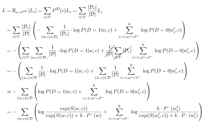
Fig. 2: The detailed calculation steps for the overall NCE loss.
Asymtopic Analysis: Why NCE works?
Recall the final expression of \(L_c\), we rewrite it to the negative sum of two expectations with simplified terms as:
\[L_{c} = - \sum_{w \in V} P^{\mathcal{D}_c} \log \frac{P^+}{P^+ + k \cdot P^-} - k \cdot \sum_{w' \in V} P^-(w') \log \frac{k \cdot P^-}{P^+ + k \cdot P^-}\]To see why NCE works, we need to compute its gradient and compare it with the gradient of the negative log-likehood function. For clearer presentaiton, we divide the calculation into two parts with the first part including the terms involving positive samples and the second part including the negative ones. Note that we can interchange \(P^{\mathcal{D}_c}\) and \(P^+\) to help with the calculation . Let \(LHS\) and \(LHS'\) denote the gradients of the first half and the second half, respectively (\(\nabla L_c = - LHS - LHS'\)), then we have:
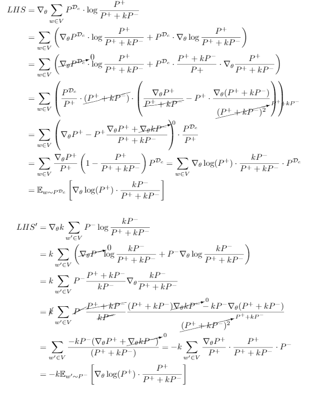
Fig. 3: The detailed calculation steps for the gradient of the NCE loss (divided into two parts for better comprehension) which is omitted in the original paper.
By combining the results, we can express the NCE loss as:
\[\begin{aligned} \nabla_{\mathcal{\theta}} L_c &= - \sum_{w \in V} \nabla_{\mathcal{\theta}}\log(P^+) \cdot \frac{kP^-}{P^+ + kP^-} \cdot P^{\mathcal{D}_c} - (-k) \sum_{w' \in V} \nabla_{\mathcal{\theta}}\log(P^+) \cdot \frac{P^+}{P^+ + kP^-} \cdot P^- \\ &= -\sum_{w \in V} \nabla_{\mathcal{\theta}}\log(P^+) \cdot \frac{kP^- P^{\mathcal{D}_c} - k P^- P^+}{P^+ + kP^-} = -\sum_{w \in V} \frac{kP^-}{P^+ + kP^-} \cdot (P^{\mathcal{D}_c} - P^+) \nabla_{\mathcal{\theta}} \cdot \log(P^+) \\ \end{aligned}\]As \(k \to \infty\), \(\nabla_{\mathcal{\theta}} L_c \to -\sum_{w \in V} (P^{\mathcal{D}_c} - P^+) \nabla_{\mathcal{\theta}} \cdot \log(P^+)\) which is the gradient of the negative log-likelihood scaled by the difference between the true data distribution and the model’s distribution. To interpret this further, we see that the extreme points will be attained with the zero gradient, i.e. either \(P^{\mathcal{D}_c} - P^+ = 0\) or the gradient of the log likelihood of our model gets zero. The former means our model perfectly fits to the data distribution and the latter suggests the maximization of our model’s log-likelihood. In other words, as the ratio of noise samples to observations increases, the negative of the NCE gradient approaches the maximum likelihood gradient.
Negative Sampling
Negative Sampling can be viewed as a special case of NCE when (1) \(k = \lvert V \rvert\) and (2) \(P^-\) is uniform. To see this, recall the monte-carlo-estimated form of the NCE loss and apply the substitutions of \(k = \lvert V \rvert\) and \(P^-(w) = \frac{1}{\lvert V \rvert}\), then we have:
\[\begin{aligned} L &= - \sum_{(w, c) \in \mathcal{D}} \left( \log \frac{\exp(S(w, c))}{\exp(S(w, c)) + \lvert V \rvert \cdot \frac{1}{\lvert V \rvert}} + \sum_{i=1, w' \sim P^-}^{\lvert V \rvert} \log \frac{\lvert V \rvert \cdot \frac{1}{\lvert V \rvert}}{\exp(S(w_i', c)) + \lvert V \rvert \cdot \frac{1}{\lvert V \rvert}} \right)\\ &= - \sum_{(w, c) \in \mathcal{D}} \left(\log \frac{\exp(S(w, c))}{\exp(S(w, c)) + 1} + \sum_{i=1, w' \sim P^-}^{\lvert V \rvert} \log \frac{1}{\exp(S(w'_i, c)) + 1} \right) \\ &= - \sum_{(w, c) \in \mathcal{D}}\left( \log \frac{1}{1 + \exp(-S(w, c))} + \sum_{i=1, w' \sim P^-}^{\lvert V \rvert} \log \frac{1}{1 + \exp(S(w'_i, c))}\right) \\ &= - \sum_{(w, c) \in \mathcal{D}}\left( \log \sigma[S(w, c)] + \sum_{i=1, w' \sim P^-}^{\lvert V \rvert} \log \sigma[-S(w'_i, c)] \right) \end{aligned}\]where \(\sigma{\cdot}\) is the sigmoid function. To interpret \(P^-\) as a uniform distribution, consider the whole corpus with each position having a “unique” token (the uniqueness is in terms of the position, not the word), it is clear that these “unique” tokens are uniformly distributed because each one of them has only one occurrence.
Tackling the Normalizing Constant Directly
All the approaches discussed in the previous sections attempt to approximate the normalizing constant, but circle around this goal with many additional settings. A natural question to ask is, why don’t we give a treatment to the normalizing constant more directly?
Self Normalization
The idea of self-normalizing softmax is to encourage the network to learn \(Z(c) = 1 \implies \log Z(c) = 0\) [7]. To achieve this, it has the following objective function:
\[\begin{aligned} L &= - \sum_{(w, c) \in \mathcal{D}} \left[ \log P(w|c) - \alpha (\log Z(c) - 0)^2\right] \\ &= - \sum_{(w, c) \in \mathcal{D}} \left[ \log P(w|c) - \alpha \log^2 Z(c)\right] \end{aligned}\]And at the decoding time, we can simply discard \(Z(c)\) in \(P(w \vert c)\) such that \(P(w \vert c) \approx \exp[S(w, c)]\) because our model has learnt \(\log Z(c) \approx 0\). The author claimed that self-normalization increases the decoding speed by a factor of \(\sim 15 \times\) for their implementation of the language model.
Note: Compared to the equation in the original paper [7] which is to maximize the log-likelihood, we add the minus sign here which instead suggests minimization for consistency in this post. Moreover, the variables are replaced as in the scenario of learning word representations or language modelling.
There are two important points to discuss here: (1) there is some freedom for \(Z(c)\) in self-normalizing softmax, compared to what is assumed in NCE (\(Z(c)\) is strictly equal to \(1\)); (2) the proposed self-normalization technique does not save the training time because the model needs to learn how to force \(Z(c) \to 1\) during training.
Note: The second point disagrees with Ruder’s post [1] where he suggested that self-normalization works for accelerating the training speed.
Sampling-based Self-Normalization
To improve the computational efficiency in the training time, Andreas and Klein (2015) [9] proposed a sampling-based self-normalization model based on the observation that as long as a sufficiently large fraction of training examples are normalized, there will be some guarantee of high probability for \(Z(c) \approx 1\) on the remaining training examples as well. Thus, the objective function was modified to the following:
\[L = - \sum_{(w, c)\in \mathcal{D}} \log P(w|c) + \frac{\alpha}{\gamma} \sum_{c' \in \mathcal{D}' \subseteq \mathcal{D}} \log^2 Z(c)\]where \(\mathcal{D}'\) is the sampled subset of our corpus \(\mathcal{D}\) and \(\gamma < 1\) is the sampling rate such that \(\lvert \mathcal{D}' \rvert = \gamma \lvert \mathcal{D} \rvert\).
Conclusions
This post focuses on the theoretical side of the softmax family, with less practical results presented. A possible future work is to write a post for more practical purposes such as some real implementation and coding details or at least summarize the softmax variants used by the well-known language models and feature representation learning techniques.
Note: The central question to be tackled by all the softmax variants in this post is to avoid expensive computation on the normalizing consant \(Z(c)\).
Acknowledgements
This post follows the same order of introducing the softmax variants as in Ruder’s post [1], but it is more mathematically inclined while lacking some discussion of the practical sides. The theories involved in this post are based on the conference papers ([2] - [7]) but the corresponding proofs are all written by myself. Thanks for Yixuan He’s effort of proofreading and review.
Citation
@misc{yuan2020softmaxvariants,
  author = {He, Yuan},
  title = {Softmax and its Variants},
  year = {2020},
  howpublished = {\url{https://lawhy.github.io//softmax-variants/}},
}
References
-
[1] Sebastian Ruder. On word embeddings - Part 2: Approximating the Softmax. http://ruder.io/word-embeddings-softmax, 2016.
-
[2] Morin, F. and Yoshua Bengio. “Hierarchical Probabilistic Neural Network Language Model.” AISTATS (2005).
-
[3] Chen, Wenlin, David Grangier and M. Auli. “Strategies for Training Large Vocabulary Neural Language Models.” ACL (2016).
-
[4] Bengio, Yoshua and Jean-Sébastien Senecal. “Quick Training of Probabilistic Neural Nets by Importance Sampling.” AISTATS (2003).
-
[5] Gutmann, M. & Hyvärinen, A.. (2010). Noise-contrastive estimation: A new estimation principle for unnormalized statistical models. Proceedings of the Thirteenth International Conference on Artificial Intelligence and Statistics, in PMLR 9:297-304
-
[6] Mnih, A. and Y. Teh. “A fast and simple algorithm for training neural probabilistic language models.” ICML (2012).
-
[7] Devlin, J., Rabih Zbib, Zhongqiang Huang, Thomas Lamar, R. Schwartz and J. Makhoul. “Fast and Robust Neural Network Joint Models for Statistical Machine Translation.” ACL (2014).
-
[8] Goldberger, J. and Oren Melamud. “Self-Normalization Properties of Language Modeling.” ArXiv abs/1806.00913 (2018): n. pag.
-
[9] Andreas, Jacob and D. Klein. “When and why are log-linear models self-normalizing?” HLT-NAACL (2015).