Though RNNs are capable of capturing sequential information, they suffer from the long-distance dependency problem when the sequence gets longer. The attention mechanism is able to capture the dependency regardless of the distance, but the positional information will be lost. While the attention mechanism can strengthen RNNs, there is a natural question: Why don’t we rely fully on the attention mechanism and, meanwhile, use some technique to preserve the positional information?
As stated in the title of the paper which proposed the powerful transduction model, Transformer, we do not need any recurrence or convolution to achieve the sequential predictions—all we need is attention.
Transformer is the first transduction model relying entirely on self-attention to compute representations of its input and output without using sequence- aligned RNNs or convolution [1].
This post is intended to guide your attention, step by step, to understand the architecture of Transformer.
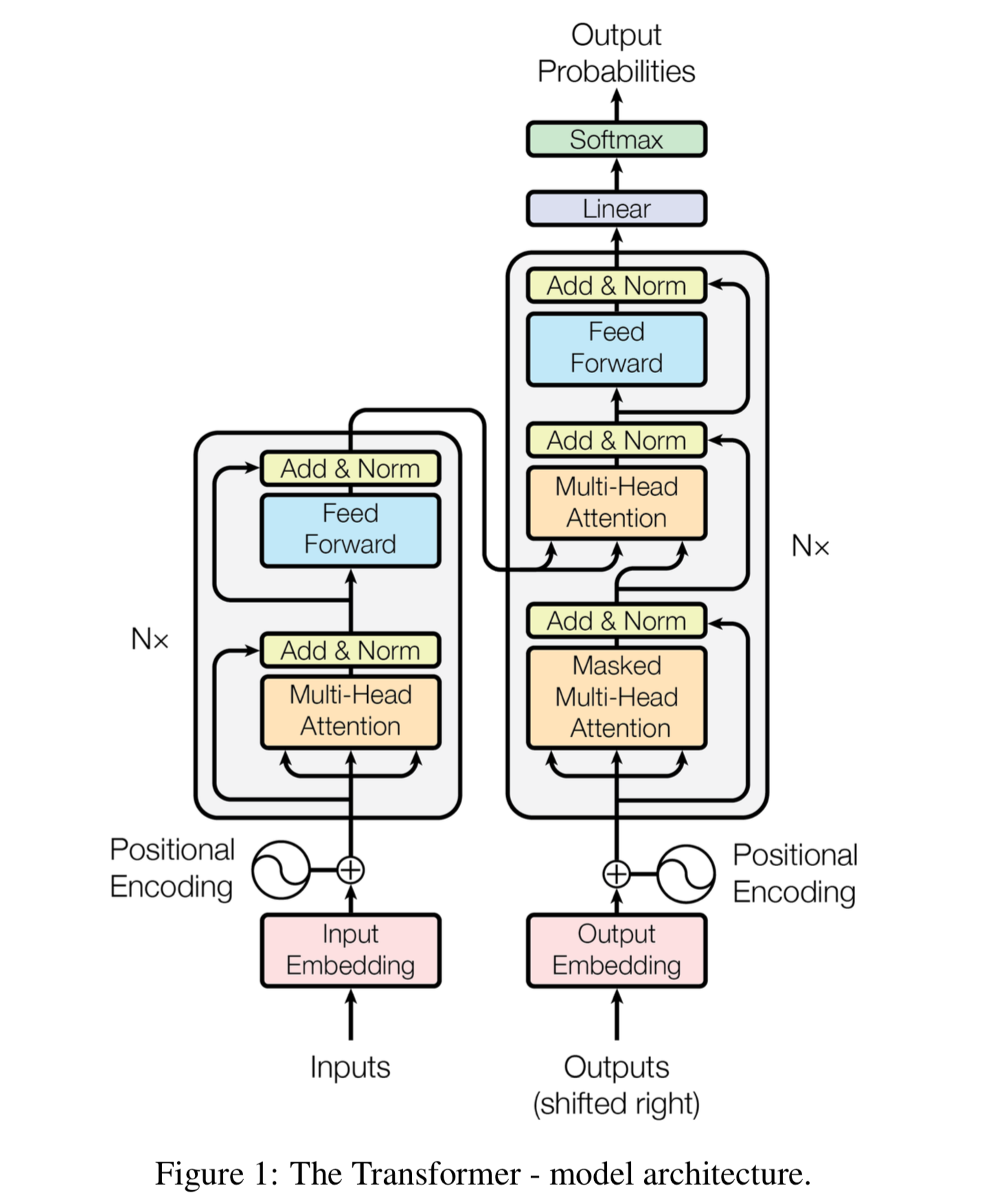
Fig 1. The model architecture of the transformer taken from the original paper [1].
In Figure 1, we can see that the overall architecture follows the encoder-decoder structure with the left half being the stacked encoder and the right half being the stacked decoder. We will go through all the components in this figure as to understand it thoroughly.
Stacked Layers
The symbol Nx means the stack of \(N\) identical layers. To overcome the problem brought by the deep architecture, the output of each sub-layer is augmented with a residual connection followed by layer normalization (Add & Norm). In short, the residual connection channels the information of the input to the deep layers and the layer normalization normalizes along the feature dimension for more stable gradients.
Multi-Head Attention
The Multi-Head Attention block employs the self-attention mechanism, which allows the model to associate each word in the input with the rest, so as to learn the compact representation of the input sequence.

Fig 2. Illustration of the Multi-Head Attention block [2].
Suppose the \(i^{th}\) input sequence is the query \(Q_i\); we want to compare it with a set of keys \(K_i\), which in our context refers to the \(i^{th}\) input sequence as well. We use the scaled dot-product to compute the similarity score between them as: \(\frac{Q_i K_i^T}{\sqrt d_{k_i}}\), where \(d_{k_i}\) is the dimension of the keys. We can pack the queries into a batch and mask out the scores of the extra paddings of the shorter sentences; then compute the score matrix as: \(\frac{Q K^T}{\sqrt d_k}\). This step corresponds to the MatMul\(\to\)Scale block in Figure 2.The reason for adding the scaling factor stated in the original paper is shown below:
We suspect that for large values of \(d_k\), the dot products grow large in magnitude, pushing the softmax function into regions where it has extremely small gradients. To counteract this effect, we scale the dot products by \(\frac{1}{\sqrt{d_k}}\) [1].
Next, we compute the attention weights by feeding the scaled dot-product scores into the SoftMax layer with the sum of each row (word) equal to \(1\) (see Figure 3).

Fig 3. The softmax of the scaled dot-product scores [2].
We then apply the weight matrix (through MatMul block) to the set of values V, which again, refers the input sequence. The softmax weights reflect the importance of each word in the input.
To achieve multi-head attention, we perform \(H\) times linear transformations on the same \(Q\), \(K\) and \(V\) with independently learned matrices. The three Linear blocks correspond to the separate (query, key and value) linear transformations of the input sequence with the matrices \(W_h^Q \in \mathbb{R}^{d_{model}\times d_k}\), \(W_h^Q \in \mathbb{R}^{d_{model}\times d_q}\) and \(W_h^V \in \mathbb{R}^{d_{model}\times d_v}\), respectively, where the subscript \(h\) refers to the \(h^{th}\) head and \(d_q = d_k\) for performing the dot-product. The expression of the multi-head attention is presented as:
The output is formed by the linear transformation of the concatenation of the \(H\) heads, with the matrix \(W^O \in R^{H d_v \times d_{model}}\). The author suggests to set \(d_k =\) \(d_v =\)\(d_{model}/H\) reduce the computational cost to the case of single-head attention with full dimensionality [1]. The applications of the multi-head attention in Transformer are summarised as follows:
-
In the encoder (
Multi-Head Attentionblock in the bottom left of Figure 1), the input sequence comes from the output of the previous encoder layer. Because of the self-attention mechanism. \(Q\), \(K\) and \(V\) refer to the same thing. As the result, each position in the encoder can attend to all positions in the previous layer of the encoder -
In the encoder-decoder attention layers (
Multi-Head Attentionblock in the central right of Figure 1), \(Q\) comes from the previous decoder layer while \(K\) and \(V\) refer to the encoder’s outputs. As such, we can predict the next output token according to the inputs’ hidden representation weighted by all the previous output tokens. -
In the decoder (
Masked Multi-Head Attentionblock in the bottom right of Figure 1), the input sequence comes from the previous decoder layer. The self-attention layers allow each position in the decoder to attend to all positions in the decoder up to and including that position. To preserve this auto-regressive property, the unseen tokens are masked out (setting to \(-\infty\)) in the scaled dot-product attention. The masking process can be achieved by adding the look-ahead mask matrix and the scaled scores as shown in Figure 4. As such, the softmax outputs of the masked positions will be zero because \(e^{-\infty} = 0\).It is important to notice the
shifted rightblock in the decoder part, which means we feed the output embedding sequentially same as in the RNN-based encoder-decoder model.

Fig 4. The masking process in the self-attention layers of the decoder up to some time step t [2].
Position-wise Feed-forward Networks
The Feed Forward blocks in both the encoder and the decoder refer to the position-wise fully connected feed-forward network, i.e. for each position, we apply the feed-forward process independently and identically. Each process consists of Linear \(\to\) Activation \(\to\) Linear. We can aggregate all of these processes with the following expression when choosing RELU as our activation:
where \(W_1 \in \mathbb{R}^{d_{model} \times d_{ff}}\) and \(W_2 \in \mathbb{R}^{d_{ff} \times d_{model}}\). Note that each position of \(x\) corresponds to a different set of parameters. As suggested by the author, another way of describing this is as two convolutions with kernel size 1 [1].
A critical note here is that the positions’ concept is the same in both the encoder and the decoder, i.e., the tokens’ positions in the input sequence. The reason is that the feed-forward network’s input is the weighted hidden representation of the input sequence coming either from the encoder’s self-attention process or the encoder-decoder-attention layer.
Weight Tying (Optional)
The author suggests that we can share the weight matrix of the learned linear embedding mapping \(E_{dec}\) with the pre-softmax linear classifier mapping \(O\), i.e. let \(E_{dec} = O^T\), with the shape of \(\vert V \vert \times d_{model}\) where \(\vert V \vert\) is the vocab size and \(d_{model}\) is the embedding dimension. In this way, the output embedding layer \(E_{dec}\) transforms the output tokens into the output embeddings, and the linear classifier \(O\) reveres the process. Finally, the softmax layer yields more confident scores on the predicted output tokens.
The author also suggests that the input embedding layer can share the same weights as \(E_{enc} = E_{dec} = O^T\). In my understanding, there are two scenarios for this option: (1) the language model tasks that use the same vocabulary space in both ends; (2) the unified vocab space formed by merging the input and output vocabs.
To counteract the scaling factor in the attention layers, the author suggests to multiply the weights in the embedding layers by \(\sqrt{d_{model}}\).
The techniques discussed in this section are design choices.
Positional Encoding
To amend the loss of the positional information in all the attention layers, we need some form of positional encoding to distinguish a word at different positions. The simplest idea is to let \(PE = pos\)\(\in \{0, 1, ..., T-1 \}\) where \(pos\) is the position/time-step of the current word and \(T\) is the length of the input sequence. But this will result in the unboundedness of the positional values because \(\sup(pos) \to \infty\). To address this problem, we could normalize the values as \(PE = \frac{pos}{T - 1}\) such that \(0 \leq PE \leq 1\). But the distance intervals are not consistent across input sentences of different lengths. Ideally, we need \(PE\) to satisfy the following criteria [3]:
-
Unique encoding for each position/time-step;
-
Adaptive to arbitrary input length;
-
Bounded values;
-
Consistent distance interval between any two positions;
Here the consistency means that for any two positions \(pos_i\) and \(pos_j\), \(PE(pos_j) - PE(pos_i)\) must be consistent across input sentences of different lengths—it does not necessarily imply that \(\forall i, j.\) \(PE(pos_j) - PE(pos_i) = C\) where \(C\) is some constant.
-
Deterministic.
The author suggests to use \(\sin\) and \(\cos\) functions to encode the positional information as they meet the criteria above. Note that the input embedding matrix has the shape of \(L \times d_{model}\) where \(L\) is the sequence length. The positional encoding matrix has the same shape as the input embedding matrix, and for each embedding dimension \(k\), it has a slightly different encoded value. The expression of the positional encoding is as follows:
\[PE[pos, k] = \begin{cases} \sin(\frac{pos}{10000^{2i/d_{model}}}) & k=2i=0,2,4,...,d_{model}-2 \\ \cos(\frac{pos}{10000^{2i/d_{model}}}) & k=2i+1=1,3,5,...,d_{model}-1 \\ \end{cases}\]where \(i \in [0,...,\frac{d_{model}}{2})\) with \(d_{model}\) a even number. The matrix form of the positional encoder is thus:
\[PE = \begin{bmatrix} \sin(\frac{1}{10000^{0/d_{model}}}) & \ldots & \sin(\frac{T}{10000^{0/d_{model}}})\\ \cos(\frac{1}{10000^{0/d_{model}}}) & \ldots & \cos(\frac{T}{10000^{0/d_{model}}})\\ \vdots & \ddots & \vdots\\ \sin(\frac{1}{10000^{(d_{model}-2)/d_{model}}}) & \ldots & \sin(\frac{T}{10000^{(d_{model}-2)/d_{model}}})\\ \cos(\frac{1}{10000^{(d_{model}-2)/d_{model}}}) & \ldots & \cos(\frac{T}{10000^{(d_{model}-2)/d_{model}}})\\ \end{bmatrix}^T\in [-1, 1]^{L \times d_{model} }\]Note that the scaling factor \(\frac{1}{10000^{2i/d_{model}}}\) decreases as the embedding dimension increases. This results in a decrease of the value change in the deeper dimension. In the post of Kazemnejad [3], he suggests that the intuitive interpretation of this behaviour is to think of the bit encoding, where the rate of change of the bit decreases as we shift to the higher bit position.
Another advantage of the proposed positional encoding is that for any fixed offset \(\delta\), \(PE[pos+\delta, ] = f(PE[pos, ])\) where \(f\) is a linear function of \(PE[pos, ]\). To see this, let \(F\) be the corresponding linear transformation matrix of the shape \(d_{model} \times d_{model}\). The equation holds if we can find a \(pos\)-independent solution \(F_k \in \mathbb{R}^{2\times2}\) for the following:
\[F_k \begin{bmatrix} \sin(w_k \cdot pos) \\ \cos(w_{k+1} \cdot pos) \end{bmatrix} = \begin{bmatrix} a & b \\ c & d \end{bmatrix} \begin{bmatrix} \sin(w_k \cdot pos) \\ \cos(w_{k+1} \cdot pos) \end{bmatrix} = \begin{bmatrix} \sin(w_{k} \cdot (pos + \delta)) \\ \cos(w_{k+1} \cdot (pos + \delta)) \end{bmatrix}\]where \(w_k\) is the scaling factor at an even dimension \(k\), and by definition, \(w_{k} = w_{k+1}\). If \(F_{k}\) exists, then \(F\) can be derived by concatenating all the submatrices \(F_k\). The following proof is largely based on Kazemnejad’s post [3].
Proof: Using the trigonometric addition formulas we have:
\[\begin{bmatrix} a & b \\ c & d \end{bmatrix} \begin{bmatrix} \sin(w_k \cdot pos) \\ \cos(w_{k+1} \cdot pos) \end{bmatrix} = \begin{bmatrix} \sin(w_{k} \cdot pos)\cos(w_k \cdot \delta) + \cos(w_k \cdot pos) \sin(w_k \cdot \delta) \\ \cos(w_{k} \cdot pos)\cos(w_k \cdot \delta) - \sin(w_{k} \cdot pos)\sin(w_k \cdot \delta) \end{bmatrix}\]Thus, we have the following equations:
\[\begin{aligned} a \sin (w_k \cdot pos) + b \cos(w_{k} \cdot pos) &= \sin(w_{k} \cdot pos)\cos(w_k \cdot \delta) + \cos(w_k \cdot pos) \sin(w_k \cdot \delta) \\ c \sin (w_k \cdot pos) + d \cos(w_{k} \cdot pos) &= - \sin(w_{k} \cdot pos)\sin(w_k \cdot \delta) + \cos(w_{k} \cdot pos)\cos(w_k \cdot \delta) \end{aligned}\]By comparing the terms on both sides, we have found \(a, b, c\) and \(d\) independent of \(pos\) such that:
\[F_k = \begin{bmatrix} cos(w_k \cdot \delta) & sin(w_k \cdot \delta)\\ -sin(w_k \cdot \delta) & cos(w_k \cdot \delta) \end{bmatrix}\]The end.
References
- [1] Vaswani, A., Shazeer, N., Parmar, N., Uszkoreit, J., Jones, L., Gomez, A. N., Kaiser, U., & Polosukhin, I. (2017). Attention is All You Need. Proceedings of the 31st International Conference on Neural Information Processing Systems, 6000–6010.
- [2] Phi, Michael. “Illustrated Guide To Transformers- Step By Step Explanation”. Medium, 2020, link.
- [3] Kazemnejad, Amirhosein. “Transformer Architecture: The Positional Encoding - Amirhossein Kazemnejad’s Blog”. Kazemnejad.Com, 2021, link.